Training a Custom YOLO Model From Scratch: From Labeled Data to a Working AI

In the previous post, we covered how to build a high-quality dataset by extracting frames from Creative Commons football footage. Now it's time to put that data to work.

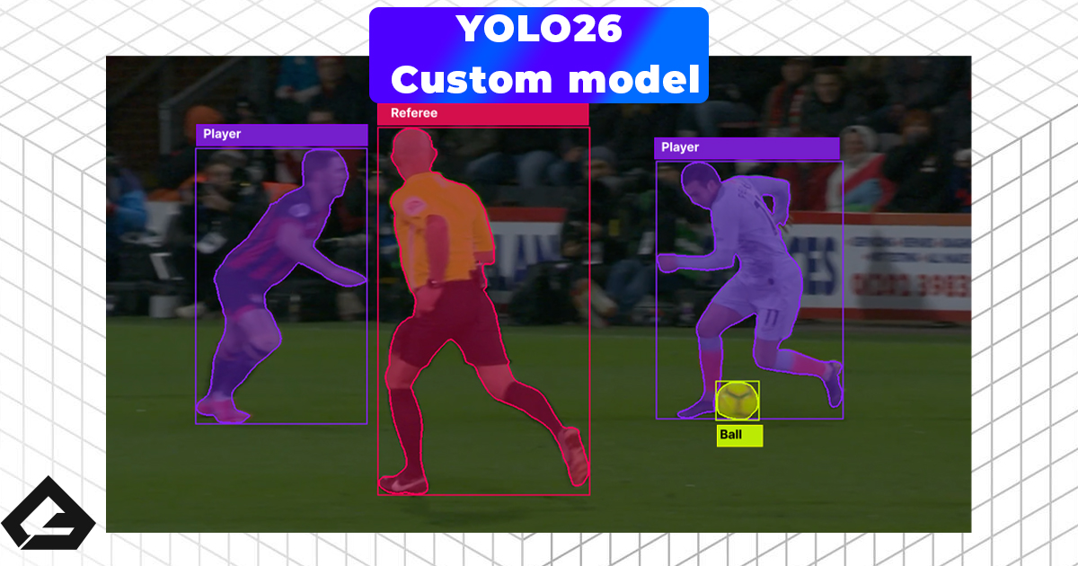
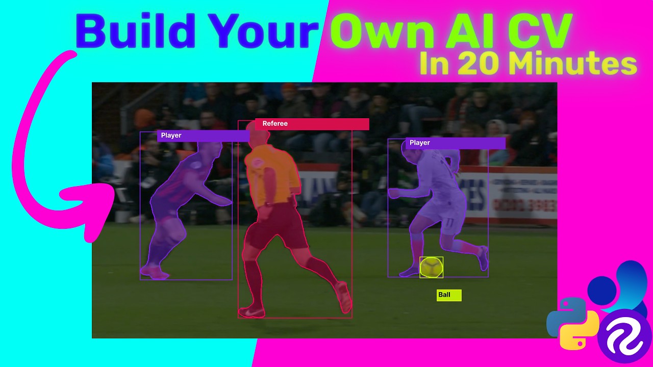
This post walks through the full pipeline: labeling your images, training a YOLOv26 model using Google Colab, and finally running that model locally on your machine. By the end, you'll have a working AI that can detect players, referees, and the ball in real time.

You can follow along with the full video tutorial here:

---

Step 1: Annotating Your Images with Roboflow

With your curated frames ready, the next step is labeling them — drawing bounding boxes around every object you want the model to detect. Doing this manually for hundreds of images is tedious, which is exactly why we use Roboflow.

Roboflow is a free platform with powerful AI-assisted labeling that dramatically speeds up the annotation process.

Setting Up Your Project

Head to roboflow.com, create a free account, and start a new project. Give it a name (e.g. football-detector), and make sure you select Object Detection as the project type.

Uploading Your Images

Upload your curated frames directly from the dashboard. Once uploaded, click Save and Continue to move into the annotation phase.

Using Auto Label

This is where Roboflow really shines. Instead of drawing boxes manually, use Auto Label with SAM 2. You'll first define your classes — the objects you want to detect. For this project:

• football — the ball
• player — any outfield player
• referee — match officials

Once your classes are set, Roboflow runs a model over your images and automatically generates bounding box annotations for each one.

Important: Auto labeling is a massive time-saver, but it isn't perfect. Think of it as a fast intern that needs a proofreader. Go through each image and approve or correct the results. The AI will occasionally miss a small ball or hallucinate a phantom player. Garbage in, garbage out — take the extra few minutes.

A confidence threshold of 40–50% works well for most objects. For small objects like a football, nudge it slightly lower to ensure it gets picked up.

Splitting and Exporting the Dataset

Once all images are approved, add them to your dataset and split them into three subsets:

• Train — 80%
• Validation — 10%
• Test — 10%

Then create a Version to lock in your work, and export it in YOLOv26 format as a .zip file. You'll upload this directly to Google Colab in the next step.

---

Step 2: Training on Google Colab

Training a computer vision model requires serious GPU power. Most people don't have a high-end AI rig at home — and that's fine. Google Colab gives you free access to a T4 GPU, which is more than enough for a prototype.

Open the training notebook here: 👉 Google Colab Training Notebook

Confirming GPU Access

In Colab, check the top-right corner — it should show your runtime as connected. If not, go to Runtime → Change Runtime Type and select T4 GPU.

Uploading Your Dataset

You have two options:

1. Upload directly into the Colab session (simple, but lost on refresh)
2. Mount Google Drive and upload there first (recommended for larger datasets)

For a quick prototype, uploading directly is fine. Once uploaded, run the extraction cell to unzip your dataset into the Colab environment automatically.

Installing Requirements

Run the cell to install the Ultralytics package — the core engine used to train, validate, and run YOLO models:

pip install ultralytics

Configuring Your Training Run

There are three key parameters to get right:

For small, fast-moving objects like a football, a higher image resolution makes a meaningful difference. 640 is the standard, but 1280 gives the model more detail to work with.

Once configured, run the training cell and grab a coffee — it typically takes around an hour on a free T4.

Retrieving Your Trained Weights

After training completes, check the runs/detect/train/weights/ folder in the sidebar. You'll see two files:

• last.pt — the final checkpoint
• best.pt — the checkpoint that performed best on your validation set

Always use best.pt for inference. Run the test cell to visually confirm the model is detecting objects correctly across your validation images.

Downloading the Model

Run the final cell to zip your weights into custom_model.zip, then right-click it in the file browser and download it to your local machine.

---

Step 3: Running the Model Locally

With your trained model downloaded, it's time to run it on your own machine. All you need is Python and a code editor — VS Code works perfectly.

Setup

Unzip custom_model.zip and open the folder in VS Code. Create a virtual environment and install dependencies:

python -m venv .venv
source .venv/bin/activate  # Windows: .venv\Scripts\activate
pip install -r requirements.txt

Your requirements.txt should include:

ultralytics
numpy
opencv-python

Writing the Inference Script

Create an index.py file. The script accepts a --source argument so you can point it at an image, a video file, or a live camera without changing the code each time:

import argparse
from ultralytics import YOLO

def main():
    parser = argparse.ArgumentParser(description="Run YOLO inference")
    parser.add_argument("--model", default="weights/best.pt")
    parser.add_argument("--source", default="media/test.png")
    args = parser.parse_args()

    if args.source == "usb":
        args.source = 0  # First connected camera

    model = YOLO(args.model)

    for result in model.predict(
        source=args.source,
        stream=True,
        show=True,
        save=True,
        project="output"
    ):
        pass

if __name__ == "__main__":
    main()

Running Inference

Test against an image:

python index.py --source media/test.png

Test against a video:

python index.py --source media/test.mkv

Run on a live USB camera:

python index.py --source usb

All results are saved to the output/ folder automatically.

---

What's Next

You now have a fully functional custom computer vision model running locally. That's no small thing.

In the next post, we're going a step further — ditching the plain bounding boxes for proper sports graphics (custom team markers, referee rings, and more), and adding advanced tracking to calculate player running speeds and ball trajectory.

Stay tuned.